
Two for One Heatmaps in R with ComplexHeatmaps
Published:
Two for One Heatmaps in R with ComplexHeatmaps
This post comes in 2 parts: gathering the data and making the heatmap.
All of the packages used in this tutorial come from Bioconductor. Start by running the following line:
source("https://bioconductor.org/biocLite.R")
Getting the Data
Basic information with biomaRt
First, if you don’t already have it installed, download ensembldb. Then, open the package and create your mart. I still use GRCh 37, but you can leave out the last argument if you are using GRCh 38.
biocLite("biomaRt") # Download
library(biomaRt) # Open package

mart <- useEnsembl(biomart="ensembl", dataset="hsapiens_gene_ensembl", GRCh=37) # Download Ensembl Biomart
Now let’s define the gene of interest and get some basic information.
gene.of.interest <- "MUC1"

gene.of.interest.info <- getBM(c("start_position", "end_position", "strand", "chromosome_name"),
                               filters="hgnc_symbol",values=gene.of.interest, mart=mart)
gene.of.interest.start <- gene.of.interest.info$start_position
gene.of.interest.strand <- gene.of.interest.info$strand
gene.of.interest.end <- gene.of.interest.info$end_position
gene.of.interest.chrom <- gene.of.interest.info$chromosome_name
LD information with Ensembl API
The Ensembl REST API allows for calls up to 500 kb, but for the purposes of speed and plotting, we will just look at 10 kb around the “half-way point” of our gene of interest.
gene.of.interest.half <- (gene.of.interest.start + gene.of.interest.end) %/% 2
start.10Kb <- gene.of.interest.half - 5000
end.10Kb <- gene.of.interest.half + 5000
The Ensembl REST API takes as parameters the chromosome of the gene of interest, the start and end position of the search range, and a population from the 1000 Genomes Project. For this tutorial, I am using the CEU population: “Utah residents with Northern and Western European ancestry”; you can find a full list of the populations here. Be aware that this is the GRCh 37 Ensembl REST API.
Since the response of the API is in json, use the “jsonlite” package. The “data.table” package is also useful because it turns the nested list returned by jsonlite into a data frame. We don’t need “httr” yet, but we may as well download it now.
install.packages(c("jsonlite", "data.table", "httr")) # Download packages

library(data.table)
library(jsonlite)
library(httr)

genomes.population <- "CEU" # Define population from 1000 Genomes project

# Request API information. Internet is needed.
LD.info.10Kb <- read_json(paste("http://grch37.rest.ensembl.org/ld/human/region/",gene.of.interest.chrom,":",
                                 start.10Kb, "..", end.10Kb -1, "/1000GENOMES:phase_3:",genomes.population,
                                 "?content-type=application/json",sep = ""))

LD.info.10Kb <- rbindlist(LD.info.10Kb, fill = FALSE) # nested list into dataframe
LD.info.10Kb$r2 <- as.numeric(LD.info.10Kb$r2)
Let’s see how many LD values got returned and see the layout of the data frame. We can also look at how many unique variants are in our LD data using a union of the variant columns. After exploring the data, we are ready to initialize a data frame that will have all the uniqe RSIDs of the variants and their base pair positions.
dim(LD.info.10Kb)
head(LD.info.10Kb)
length(union(LD.info.10Kb$variation1, LD.info.10Kb$variation2))

LD.info.10Kb.unique.variants <- data.frame(rsid = union(LD.info.10Kb$variation1, LD.info.10Kb$variation2),
                                            position = numeric(length(union(LD.info.10Kb$variation1,
                                            LD.info.10Kb$variation2))))
Fetching the variant positions from Ensembl is a bit tricky. Basically, Ensembl will only let you make 200 calls at a time, which involves some indexing fun to make sure all of the positions end up with the right variants as quickly as possible. It’s not needed for this example, but it might save you some time if you want to retrieve positions from a larger area. After fetching the positions, we will sort all of the variants by bp position.
# Fetch Position from Ensembl using RSID
server <- "http://grch37.rest.ensembl.org"
ext <- "/variation/homo_sapiens"
i <- 1
while(i < dim(LD.info.10Kb.unique.variants)[1]){
  j <- i + 190 # Ensembl takes at most 200 requests at a time.
  if(j > dim(LD.info.10Kb.unique.variants)[1]){
    j = dim(LD.info.10Kb.unique.variants)[1]
  }
  rest.api.response <- r <- POST(paste(server, ext, sep = ""), content_type("application/json"), accept("application/json"),
                                 body = paste('{ "ids" : [', paste0(LD.info.10Kb.unique.variants$rsid[i:j],
                                                                    collapse = "\",\""), ' ] }', sep = "\""))
  rest.api.info <- fromJSON(toJSON(content(rest.api.response)))
  for(k in 1:length(rest.api.info)){
    LD.info.10Kb.unique.variants$position[k + i - 1] <- rest.api.info[[k]]$mappings$start[[1]]
  }
  i <- j + 1
}

# Get rid of 0s if applicable and sort ascending by position
LD.info.10Kb.unique.variants <- LD.info.10Kb.unique.variants[which(LD.info.10Kb.unique.variants$position > 0),]
LD.info.10Kb.unique.variants <- LD.info.10Kb.unique.variants[order(LD.info.10Kb.unique.variants$position),]
Now that we have all of the information we need, we can create the R-squared matrix for LD.
LD.r2.10Kb <- matrix(0,nrow = dim(LD.info.10Kb.unique.variants)[1], ncol= dim(LD.info.10Kb.unique.variants)[1],
                     dimnames = list(LD.info.10Kb.unique.variants$rsid, LD.info.10Kb.unique.variants$rsid))
# populate the r2 matrix
for(i in 1:dim(LD.info.10Kb)[1]){
  LD.r2.10Kb[LD.info.10Kb$variation1[i], LD.info.10Kb$variation2[i]]<-
    LD.r2.10Kb[LD.info.10Kb$variation2[i],LD.info.10Kb$variation1[i]] <-
    LD.info.10Kb$r2[i]
}
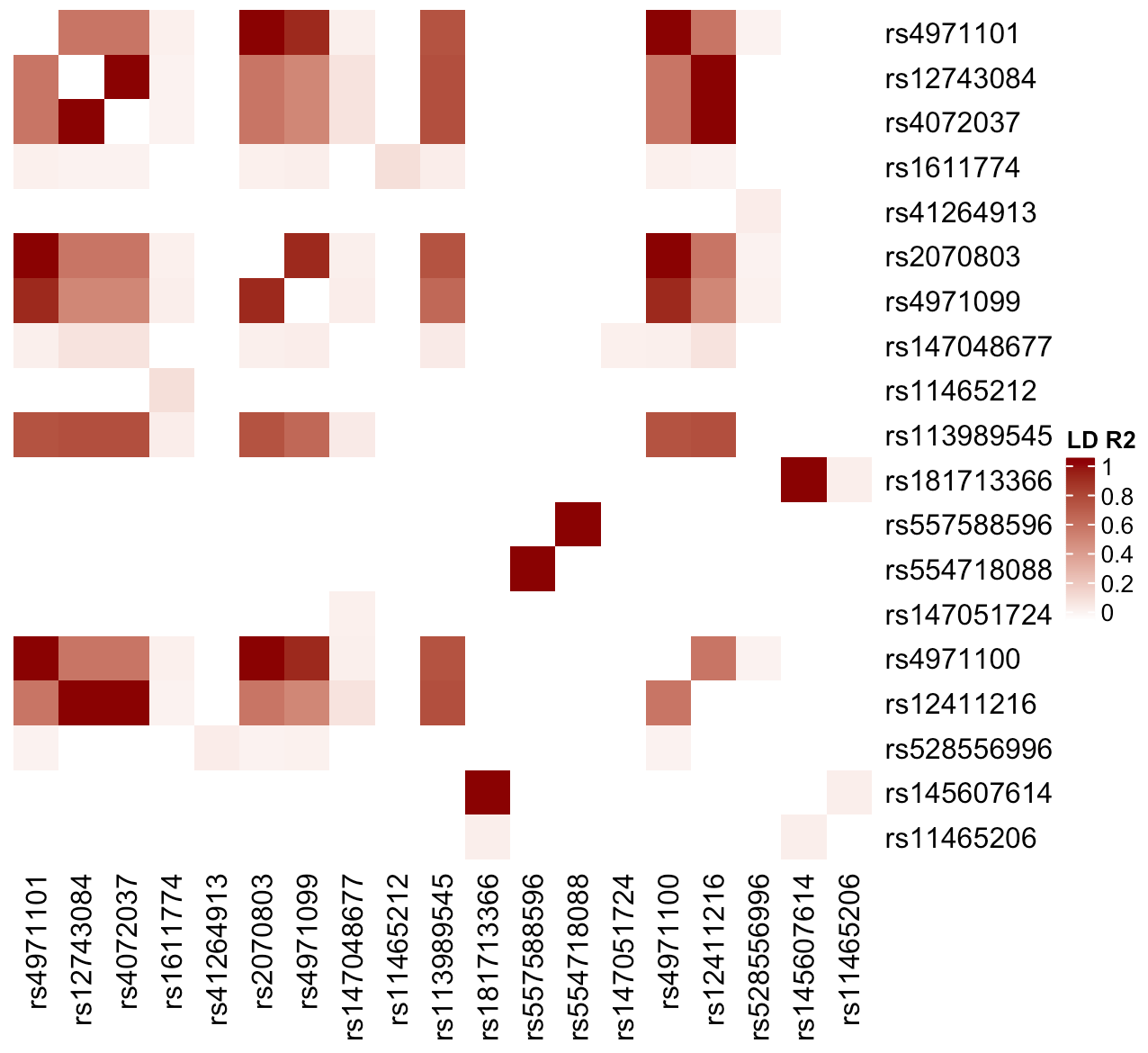
Let’s make a Heatmap with just the R-squared values.
Heatmap(LD.r2.10Kb, name = "LD R2" col = colorRamp2(c(0,1), c("white", "darkred")), cluster_rows = FALSE,
cluster_columns = FALSE, show_row_names = TRUE, show_column_names = TRUE, show_column_dend = FALSE)
Thanks to the handy function outer(), we can generate a matrix with the bp position differences between variants in one line.
LD.dist.10Kb <- outer(LD.info.10Kb.unique.variants$position, LD.info.10Kb.unique.variants$position, "-")
Since we want to show both LD and distances on the same heatmap, we can zero the out half of each matrix. The R-squared values are already betweem zero and one, but it is also nice to scale the distances to be between zero and one for the heatmap.
LD.r2.10Kb[lower.tri(LD.r2.10Kb)] = 0
SORRY THIS ISN’T DONE YET :(